Generate spectra · Payne Zero

Start with one stellar state and one wavelength window

Every calculation needs an effective temperature, surface gravity, composition, microturbulence, wavelength interval, numerical wavelength sampling, and execution device. Keeping these choices together makes the later distinction between atmosphere and spectrum generation easier to follow.

import numpy as np
import torch

from payne_zero_atmosphere import solve_structured_atmosphere
from payne_zero_synthesis import synthesize, synthesize_from_labels

device = (
    "cuda" if torch.cuda.is_available()
    else "mps" if torch.backends.mps.is_available()
    else "cpu"
)
torch_dtype = torch.float32 if device == "mps" else torch.float64
dtype = "float32" if device == "mps" else "float64"

solar_state = dict(
    effective_temperature=5777.0,
    log_surface_gravity=4.44,
    microturbulence_km_s=1.0,
)

solar_window = dict(
    wavelength_start_nm=500.0,
    wavelength_end_nm=502.0,
    r_grid=300_000,
    device=device,
    dtype=dtype,
)

device="auto" is also accepted. The explicit selection above is useful in a notebook because it makes the numerical type visible: Apple Metal uses float32, while the CUDA and CPU examples use float64 unless another supported type is requested.

The wavelength limits are vacuum nanometers. Here, r_grid=300_000 controls the logarithmic sampling of the intrinsic calculation. It is a numerical grid choice, not a claim about the resolving power of a later instrument.

Related sourceSynthesis API · Device selection

Choose how to describe the chemical composition

The abundance inputs determine the complete elemental mixture used by the atmospheric structure, particle populations, and opacity. Payne Zero accepts three descriptions. This choice is independent of the next choice—whether to hold the predicted atmosphere fixed or iterate it to convergence.

Bracket abundances are logarithmic comparisons with the Sun. [M/H] describes the overall metal-to-hydrogen ratio, [X/H] describes one element X relative to hydrogen, and [X/M] describes that element relative to the bulk metal content. A change of +1 dex means a factor of ten; −0.5 dex means about one third of the solar ratio.

Use a bulk metallicity and shared alpha pattern

This is the default for ordinary stellar work. [M/H] shifts all metals together, while [α/M] adds a common offset to O, Ne, Mg, Si, S, Ca, and Ti. The Greek letter alpha names this element group; the value states how its abundance differs from the bulk metal pattern.

Let carbon, nitrogen, and oxygen vary independently

For evolved stars and other CNO-sensitive cases, add [C/M], [N/M], and [O/M] to the bulk description. These three values allow the surface CNO pattern to depart from the overall metallicity and alpha pattern. Explicit oxygen replaces the alpha-scaled oxygen value; the other alpha elements continue to follow [α/M].

This distinction matters in cool and evolved stars because CO, CN, and OH share the same elemental inventory. Changing one abundance can alter several molecular systems and the local continuum.

Specify an element-by-element mixture

Use this description when a grouped pattern is not sufficient. Provide [Fe/H] as the baseline and list only the elements that differ from it; unspecified supported metals inherit [Fe/H]. The public interface accepts individual [X/H] values for the supported elements. This mode is selected explicitly and is not mixed with [M/H], [α/M], or the grouped CNO inputs.

The element-by-element starting structure is a provisional model for rapid spectrum trials. Its spectrum is marked as requiring atmosphere convergence; run the atmosphere solver before retaining a physical result for the requested mixture.

Define the three alternatives once. The following sections pass each of them through both model-generation workflows:

bulk_mixture = dict(
    metallicity=0.0,
    alpha_enhancement=0.0,
)

giant_state = dict(
    effective_temperature=4600.0,
    log_surface_gravity=2.2,
    microturbulence_km_s=1.7,
)

cno_mixture = dict(
    metallicity=-0.4,
    alpha_enhancement=0.2,
    c_over_m=-0.25,
    n_over_m=0.35,
    o_over_m=0.15,
)

# The synthesis API accepts element symbols in x_over_h.
individual_mixture_for_synthesis = dict(
    fe_over_h=-0.4,
    x_over_h={"C": -0.65, "N": -0.05, "Mg": -0.15},
    initializer_family="direct_abundance",
)

# The atmosphere solver accepts the same [X/H] values as named keywords.
individual_mixture_for_atmosphere = dict(
    fe_over_h=-0.4,
    c_over_h=-0.65,
    n_over_h=-0.05,
    mg_over_h=-0.15,
)

infrared_window = dict(
    wavelength_start_nm=1500.0,
    wavelength_end_nm=1700.0,
    r_grid=300_000,
    device=device,
    dtype=dtype,
)

For the bulk and CNO descriptions, the same dictionary is accepted by both Python entry points. The element-by-element spelling differs slightly: synthesis accepts an x_over_h mapping, whereas the atmosphere solver accepts named values such as c_over_h. Both represent the same [X/H] abundances.

Synthesize while holding the initialized atmosphere fixed

Use synthesize_from_labels when the spectrum is the required output and the atmosphere does not need to be solved separately to convergence. The function initializes the depth structure from the requested stellar labels, then holds that structure fixed while rebuilding populations, evaluating continuous and line opacity, and solving radiative transfer.

bulk_spectrum = synthesize_from_labels(
    **solar_state,
    **bulk_mixture,
    **solar_window,
)

cno_spectrum = synthesize_from_labels(
    **giant_state,
    **cno_mixture,
    **infrared_window,
)

individual_spectrum = synthesize_from_labels(
    **giant_state,
    **individual_mixture_for_synthesis,
    **infrared_window,
)

print(bulk_spectrum.atmosphere_converged)  # False
bulk_spectrum.save_npz("runs/solar_fixed_atmosphere_spectrum.npz")

These three calls differ only in how the chemical mixture is described. Each predicts a starting atmosphere appropriate to that mixture and passes it to the same synthesis calculation.

This command-line example uses the bulk metallicity and alpha description:

payne-zero-synthesis \
  --effective-temperature 5777 \
  --log-surface-gravity 4.44 \
  --metallicity 0.0 \
  --alpha-enhancement 0.0 \
  --microturbulence-km-s 1.0 \
  --wl-start-nm 500 \
  --wl-end-nm 502 \
  --r-grid 300000 \
  --device auto \
  --out runs/solar_fixed_atmosphere_spectrum.npz

The emergent flux in all three cases is calculated by the physical synthesis engine. Its accelerator-parallel implementation is fast enough to use directly, without a label-to-flux spectral emulator. The predicted atmosphere remains fixed during synthesis and has not passed the iterative atmosphere convergence test, so each result records atmosphere_converged=False. That distinction matters when the atmosphere itself is a scientific product.

If the spectrum alone is sufficient, this is the shortest complete interface. If the atmospheric structure must satisfy hydrostatic, radiative, and convective consistency at the requested composition, continue with the same labels in the next section.

Solve the atmosphere, then synthesize from that structure

The atmosphere solver accepts the same three scientific abundance descriptions. It uses the corresponding predicted structure as a starting point, then iterates the coupled depth variables. Each pass updates pressure, populations, opacity, radiative transfer, convection, and the temperature correction. Once the configured stopping criteria are met, the solver writes a structured atmosphere archive.

bulk_atmosphere_path = solve_structured_atmosphere(
    **solar_state,
    **bulk_mixture,
    out_dir="runs/solar_atmosphere",
)

cno_atmosphere_path = solve_structured_atmosphere(
    **giant_state,
    **cno_mixture,
    out_dir="runs/cno_giant_atmosphere",
)

individual_atmosphere_path = solve_structured_atmosphere(
    **giant_state,
    **individual_mixture_for_atmosphere,
    out_dir="runs/individual_giant_atmosphere",
)

# Choose any one of the three converged archives for synthesis.
physical_spectrum = synthesize(
    cno_atmosphere_path,
    wavelength_start_nm=infrared_window["wavelength_start_nm"],
    wavelength_end_nm=infrared_window["wavelength_end_nm"],
    resolution=infrared_window["r_grid"],
    device=device,
    dtype=dtype,
)

physical_spectrum.save_npz("runs/cno_giant_physical_spectrum.npz")

The first three calls show the bulk, independent-CNO, and element-by-element alternatives. Choose the one appropriate to the star; the final synthesize call is the same for any converged archive. For the element-by-element case, the public atmosphere path returns a product only after the exact convergence conditions have been met.

From the command line, this example uses independent CNO abundances. The atmosphere output path remains explicit so the synthesis command reads the product written by the solver:

payne-zero-atmosphere \
  --effective-temperature 4600 \
  --log-surface-gravity 2.2 \
  --metallicity -0.4 \
  --alpha-enhancement 0.2 \
  --c-over-m -0.25 \
  --n-over-m 0.35 \
  --o-over-m 0.15 \
  --microturbulence-km-s 1.7 \
  --out runs/cno_giant_atmosphere

payne-zero-synthesis \
  runs/cno_giant_atmosphere/payne_zero_structured_atmosphere.npz \
  --wl-start-nm 1500 \
  --wl-end-nm 1700 \
  --r-grid 300000 \
  --device auto \
  --out runs/cno_giant_physical_spectrum.npz

synthesize reads that archive and performs the same spectrum calculation used by the label interface. The difference between these calls is the atmosphere supplied to synthesis, not a second flux model.

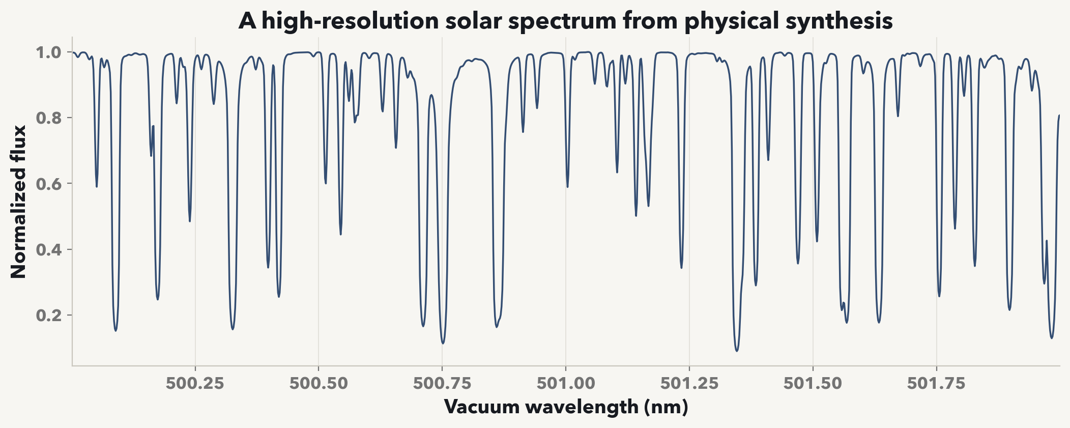
A high-resolution physical solar spectrum calculated by Payne Zero from 500 to 502 nanometers — A real Payne Zero solar calculation over 500–502 nm on the native logarithmic grid at R = 300,000. This example uses the bundled converged atmosphere. Fixed-atmosphere synthesis returns the same total-flux, continuum-flux, and normalized-flux products without implying a comparison between the two atmosphere treatments.

Keep the structured archive when you need to inspect depth quantities, reuse one atmosphere for several wavelength windows, or retain a final model whose atmospheric convergence has been checked. The file also carries convergence and source information so it can be distinguished from an intermediate starting state.

Use physical columns from another atmosphere calculation

If another solver already provides temperature, column mass, gas pressure, electron density, microturbulence, and elemental number fractions, the public builder can populate and validate those columns for Payne Zero synthesis. This is the supported bridge for an external physical atmosphere; historical text decks are not synthesis inputs.

from payne_zero_synthesis import (
    build_structured_atmosphere,
    save_structured_atmosphere,
)

external_atmosphere = build_structured_atmosphere(
    temperature=temperature_k,
    column_mass=column_mass_g_cm2,
    gas_pressure=gas_pressure_dyn_cm2,
    electron_density=electron_density_cm3,
    elemental_abundances=number_fractions_z1_to_z99,
    microturbulence=microturbulence_cm_s,
)
save_structured_atmosphere(
    external_atmosphere,
    "runs/external_atmosphere.npz",
)

Inspect and save the calculated spectrum

A spectrum contains vacuum wavelength, total surface flux density, physical continuum surface flux density, and their normalized ratio. Flux densities are reported per nanometer. All four arrays share the same final grid unless an instrument model supplies a different output grid.

for name, values in {
    "wavelength_nm": bulk_spectrum.wavelength_nm,
    "flux_total": bulk_spectrum.flux_total,
    "flux_continuum": bulk_spectrum.flux_continuum,
    "normalized_flux": bulk_spectrum.normalized_flux,
}.items():
    print(name, values.shape, np.all(np.isfinite(values)))

bulk_spectrum.save_npz(
    "runs/solar_fixed_atmosphere_spectrum.npz"
)

with np.load("runs/solar_fixed_atmosphere_spectrum.npz") as saved:
    wavelength_nm = saved["wavelength_nm"]
    normalized_flux = saved["normalized_flux"]

Save the complete product rather than only normalized flux. Total and continuum flux preserve the information needed to change normalization or apply an instrument model consistently. The saved archive also records runtime and, for a fixed-atmosphere result, the requested labels and atmosphere source information.

Keep the window fixed when generating a model sequence

Repeated calculations are simplest when wavelength limits, R, catalogs, device, and numerical type remain unchanged. Payne Zero can then reuse prepared catalog windows and device-resident invariants while only the atmospheric state and populations change.

metallicity_grid = np.array([-0.5, -0.25, 0.0, 0.25])
model_grid = []

for metallicity in metallicity_grid:
    mixture = {
        "metallicity": float(metallicity),
        "alpha_enhancement": 0.0,
    }
    model = synthesize_from_labels(
        **solar_state,
        **mixture,
        **solar_window,
    )
    model_grid.append(model.normalized_flux)

model_grid = np.stack(model_grid)
print(model_grid.shape)

The first call in a fresh environment may include compilation and cache construction. Compare steady repeated calls only after the same window has been prepared, and record the device and dtype with any timing. Changing the wavelength interval or line catalogs is a new preparation problem rather than a like-for-like repeat.

Reuse one atmosphere across several wavelength windows

When the stellar state is unchanged and only the wavelength window changes, initialize once and pass that same in-memory atmosphere tosynthesize. Do not reuse it after changing the stellar labels or abundance mixture.

from payne_zero_synthesis import (
    initialize_atmosphere_from_labels,
    synthesize,
)

initialized = initialize_atmosphere_from_labels(
    **solar_state,
    **bulk_mixture,
    device=device,
    dtype=dtype,
)

blue_window = synthesize(
    initialized,
    wavelength_start_nm=400.0,
    wavelength_end_nm=500.0,
    resolution=300_000,
    device=device,
    dtype=dtype,
)
red_window = synthesize(
    initialized,
    wavelength_start_nm=600.0,
    wavelength_end_nm=700.0,
    resolution=300_000,
    device=device,
    dtype=dtype,
)

At this point the model-generation chain is complete: a stellar state becomes either an initialized atmosphere held fixed during synthesis or a physically converged atmosphere followed by synthesis. In both paths the chosen composition enters before populations and opacity. Mapping that intrinsic spectrum to an instrument and observed pixels is the first step of the Fitting chapter.

Understand the calculationFollow the atmosphere, populations, opacity, transfer, convergence cycle, and parallel execution.