Line Calibration · Payne Zero

Calibration changes named line parameters inside synthesis

Atomic catalogs contain oscillator strengths and damping data that may be uncertain, incomplete, or inconsistent across sources. A standard-star residual can therefore contain a line-specific component even when the atmosphere, composition, continuum, and instrument model are otherwise adequate.

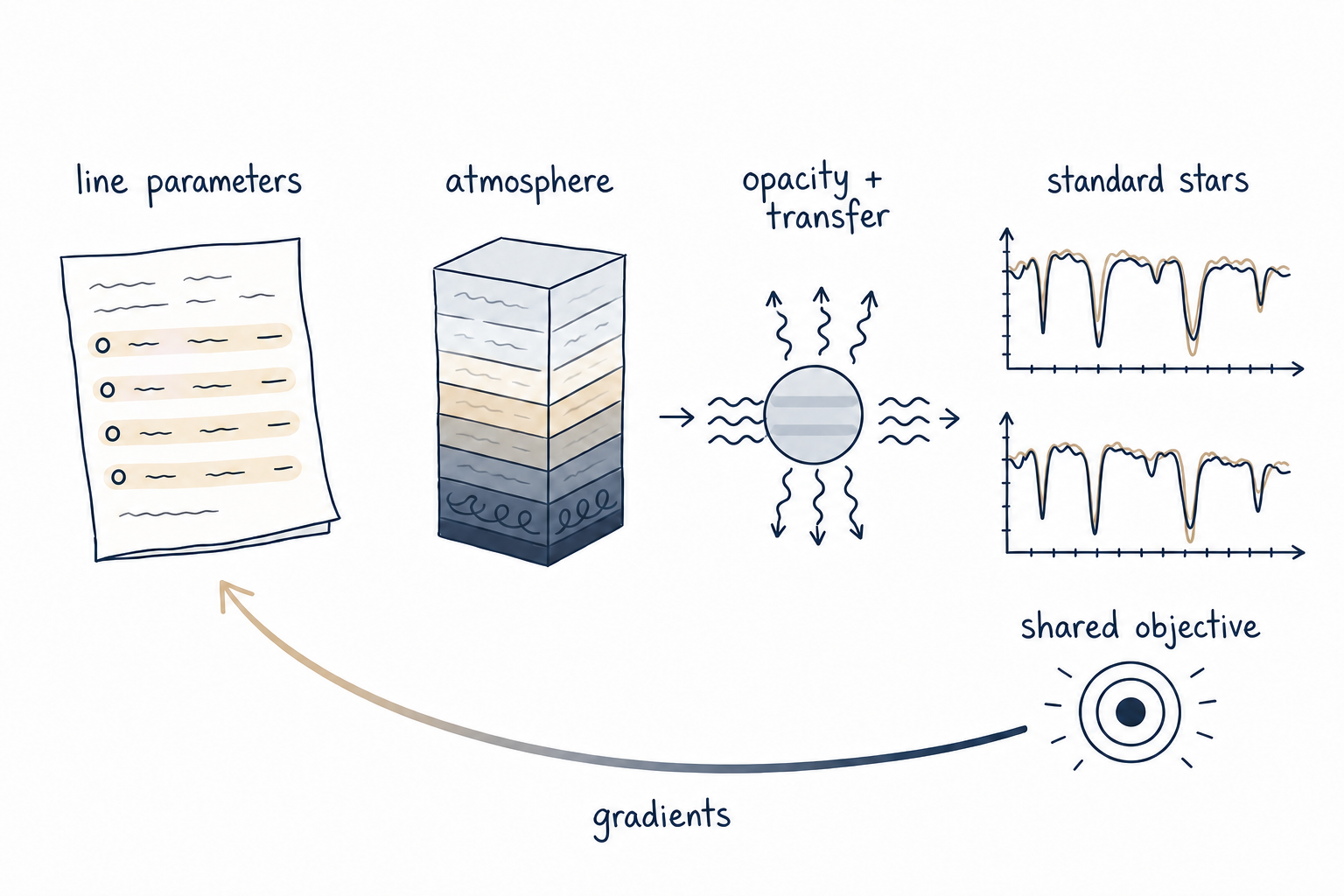
Payne Zero exposes selected catalog inputs as differentiable corrections. Each trial applies those corrections before line opacity and radiative transfer. The resulting flux is then broadened, sampled, continuum-profiled, and compared with the standard. Nothing in this workflow adds an empirical correction directly to the synthesized flux.

Selected atomic corrections propagated through opacity, radiative transfer, broadening, and sampling to standard-star residuals — The mismatch with the standard-star spectra is differentiated back to named physical catalog parameters. Atmospheres and unselected opacity remain fixed during one calibration.

Define the standards and comparison before choosing parameters

CalibrationData stores the observed standard spectra, inverse variances, masks, and any continuum bases. The physical model supplies the fixed atmosphere, wavelength window, selected transitions, velocity registration, broadening, and instrument sampling for each standard.

The bundled small example uses a real solar Fourier-transform-spectrometer excerpt and varies one Fe I oscillator strength. The larger paper experiment combines the Sun and Arcturus so that one correction set must reduce residuals in two different atmospheric conditions.

Masks and continuum freedom are part of the calibration definition. A poorly modeled blend, telluric residual, or overly flexible continuum can otherwise push a line parameter toward compensating for a different problem.

Use another standard star

A different standard uses the same boundary: one converged structured atmosphere, observed wavelength and normalized-flux arrays, weights, velocity registration, broadening, and an ordered transition list. Extend the native synthesis interval beyond the observed pixels so shifting and broadening have context.

import numpy as np

from linelist_calibration import (
    AtomicTransition,
    CalibrationConfiguration,
    CalibrationData,
    SynthesisLineCalibrationModel,
    calibrate_line_parameters,
)

data = CalibrationData(
    flux=observed_normalized_flux,
    weight=np.where(good_pixel_mask, inverse_variance, 0.0),
)
physical_model = SynthesisLineCalibrationModel(
    "runs/standard_star_atmosphere.npz",
    wavelength_start_nm=1567.9,
    wavelength_end_nm=1568.4,
    resolution=300_000,
    transitions=(
        AtomicTransition(26, 1, 1568.18024, name="Fe I 1568.180 nm"),
    ),
    observed_wavelength_nm=observed_wavelength_nm,
    radial_velocity_km_s=registered_velocity_km_s,
    gaussian_broadening_sigma_km_s=broadening_sigma_km_s,
    device="auto",
    dtype="auto",
)
configuration = CalibrationConfiguration(
    initial=np.zeros(1),
    lower=np.full(1, -1.0),
    upper=np.full(1, 1.0),
    names=("Fe I delta log(gf)",),
    maximum_iterations=30,
    device=str(physical_model.device),
    dtype=str(physical_model.dtype).removeprefix("torch."),
)
result = calibrate_line_parameters(
    data,
    configuration,
    physical_model.callback(("loggf",)),
)

Atomic number 26 denotes iron, ion stage 1 is neutral, wavelengths are in vacuum nanometers, and fitted corrections are additive dex offsets. For a joint calibration, construct one physical model per star with the same ordered transitions and concatenate their model, flux, and weight arrays in the same star order.

Each public correction has a defined catalog operation

Oscillator strength

A δ log(gf) correction is added to the catalog logarithmic oscillator strength. The correction is measured in dex, where +1 dex multiplies the oscillator strength by ten. It primarily changes the frequency-integrated line opacity and therefore line strength.

Van der Waals damping

A δ log γ_vdW correction multiplies the neutral-collision damping coefficient by 10^δ. Its strongest effect is on pressure-broadened wings.

Radiative and Stark damping

The corresponding δ log γ_rad and δ log γ_S corrections multiply natural and charged-particle damping by 10^δ. The four families can be optimized separately or in a declared joint order.

Line centers and lower excitation energies remain fixed in the demonstrated four-parameter calibration. Parameter grouping can bind multiple catalog records that represent the same physical transition so they receive one correction rather than independent values.

Each correction is propagated through the spectrum calculation

SynthesisLineCalibrationModel resolves the selected transitions against an exact source catalog and constructs a model function for the requested kinds of correction. That function returns flux in the same order as the calibration data, and PyTorch can differentiate it through opacity, transfer, broadening, and sampling.

from linelist_calibration import calibrate_line_parameters
from linelist_calibration.examples.fit_solar_fts_line import build_example

data, configuration, physical_model, atlas_metadata = build_example(
    device="auto",
    dtype="auto",
    maximum_iterations=30,
)

model = physical_model.callback(("loggf",))
result = calibrate_line_parameters(
    data,
    configuration,
    model,
)

result.save("runs/solar_fts_line_calibration")
physical_model.write_atomic_calibration_overlay(
    result.values,
    "runs/solar_fe_i_overlay.npz",
    parameter_families=("loggf",),
    calibration_name="my_solar_fe_i_calibration",
)

The observed solar FTS spectrum around Fe I 1568.180 nanometers, the spectrum from the original line data, and the spectrum after fitting the oscillator strength correction — The installed example fits one Fe I oscillator-strength correction against a real Livingston–Wallace solar Fourier-transform-spectrometer (FTS) excerpt. This view is restricted to the fitted Fe I profile, where the original line data are gray and δ log(gf) = +0.801 dex produces the orange curve. Only that named oscillator strength is varied; neighboring line data, the solar atmosphere, velocity registration, and broadening remain fixed. Residuals from those other ingredients are not expected to disappear.

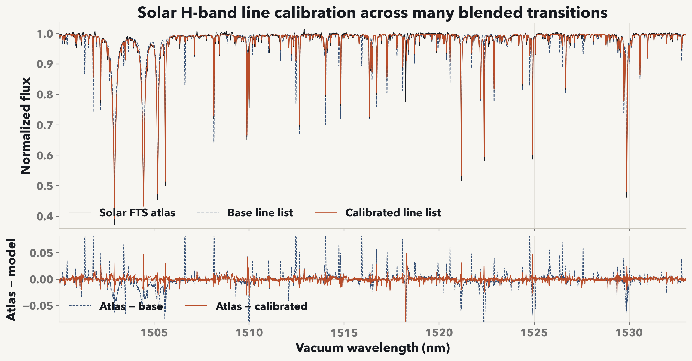
The example builder returns four separate objects: the calibration data, the bounded fitting configuration, the physical model, and metadata describing the solar atlas excerpt. Keeping these roles separate makes it possible to change a mask or fitting method without changing the source catalog or adopted atmosphere.

The same small example is installed as a command-line program:

python -m linelist_calibration.examples.fit_solar_fts_line \
  --output-dir runs/solar-fts-line-calibration

Fit the selected line corrections within physical bounds

CalibrationConfiguration declares parameter names, bounds, optional prior constraints, fitting settings, and stopping controls. calibrate_line_parameters compares all standards jointly, obtains the needed derivatives from the model, applies bounded updates, and records every accepted step inCalibrationResult.

A better fit to the calibration spectra is necessary but not sufficient. Corrections should be checked by transition group, line strength, standard, and held-out application. The paper therefore evaluates the shared Sun–Arcturus solution on a frozen APOGEE control sample rather than reporting only how well it fits the two standards.

Write corrections as an overlay, never as a silent catalog edit

The saved overlay stores the kinds and values of the corrections, the affected transitions and their grouping, a calibration name, and the SHA-256 identity of the source catalog. It contains only explicit corrections, not a loosely copied replacement line list.

import numpy as np

from linelist_calibration import (
    apply_atomic_calibration,
    validate_atomic_calibration,
)
from payne_zero_synthesis import paths as synthesis_paths
from payne_zero_synthesis.atomic_lines import load_catalog

source_catalog = synthesis_paths.source_catalog_path(
    "lines", "atomic_source_lines_parsed.npz"
)
parsed_catalog = load_catalog(
    (1567.9, 1568.4),
    300_000,
    catalog_path=source_catalog,
)
base_catalog = {
    name: value
    for name, value in vars(parsed_catalog).items()
    if isinstance(value, np.ndarray)
}

validate_atomic_calibration("runs/solar_fe_i_overlay.npz")
corrected_catalog, overlay_metadata = apply_atomic_calibration(
    base_catalog,
    "runs/solar_fe_i_overlay.npz",
    source_catalog_path=source_catalog,
)

Loading and applying an overlay validates the catalog identity and returns a corrected copy. The base catalog on disk is not modified. A digest or component mismatch stops application instead of attaching corrections to the wrong rows.

This preserves both reproducibility and reversibility: a spectrum can record the original catalog and the exact overlay, and another user can reproduce or omit that calibration without reconstructing hidden edits.

The package also provides named Sun, Arcturus, and shared Sun–Arcturus overlays through bundled_atomic_calibration. Use validate_atomic_calibration before applying an overlay in a new workflow; use write_substituted_catalog only when a complete corrected local catalog is explicitly required.

Interpret the calibration within its stated scope

A standard-star correction absorbs residuals conditional on the adopted one-dimensional atmospheres under local thermodynamic equilibrium (LTE), abundance scales, continuum treatment, masks, transition grouping, and instrument models. It is not a new laboratory measurement of oscillator strength or damping.

Testing another star or survey shows whether the correction remains useful outside the standards; it does not make the correction universal. Broader application requires additional standards, held-out spectra, appropriate priors, and renewed checks for blends, non-LTE behavior, and instrument mismatch.

Project and citationFind the source repository, authors, citation, license, and scientific lineage.