Fitting · Payne Zero

Fit the full spectrum because abundance responses are coupled

A stellar abundance is not measured only by the isolated lines carrying that element's name. Blends allow several species to affect one pixel. Magnesium and other electron donors can change the H⁻ continuum. Carbon, nitrogen, and oxygen share molecular equilibria, and a changed mixture can alter line blanketing and the atmospheric structure. A full-spectrum fit lets all retained pixels constrain these connected responses together.

Direct synthesis also makes a discrepancy easier to locate. A mismatch can enter through the stellar state, the atmosphere, line data, continuum treatment, velocity, broadening, the instrument line-spread function, or the observations themselves. Payne Zero keeps those operations separate, so a fit can test the relevant physical or instrumental cause rather than placing an empirical correction directly on the flux.

A reliable fit therefore has a definite order: define the retained pixels, project the physical spectrum through the instrument, specify the weights and continuum freedom, search the stellar parameters, and finally test the candidate with a converged atmosphere.

Begin with a model and observation on clearly defined grids

The synthesis grid is chosen to resolve the intrinsic opacity and line profiles. The observed grid is set by detector pixels and the reduction. A fit should not compare those arrays until the model has passed through the same velocity, broadening, line-spread, and sampling assumptions used for the observation.

Supply the observed wavelength and normalized flux together with the inverse variance and mask that determine each pixel's role. Leave excluded pixels in place rather than silently removing them, so the model, data, and weights retain the same indexing.NormalizedSpectrum records that observation and pixel selection in one object.

With that boundary fixed, every trial spectrum can be transformed to the same pixels before a residual is evaluated.

Project total and continuum flux through the instrument

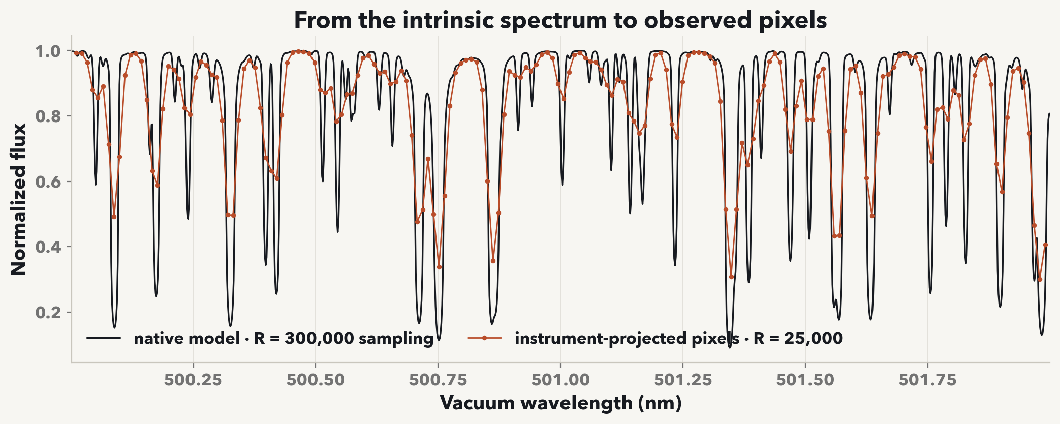
Before a residual can be meaningful, the intrinsic spectrum must be shifted, broadened, convolved with the line-spread function, and sampled on the detector grid. ObservedSpectrumOperatorperforms those operations from the logarithmic synthesis grid to any strictly increasing observed grid inside the calculated wavelength interval.

from fitter import ObservedSpectrumOperator

instrument = ObservedSpectrumOperator(
    native_wavelength_nm,
    observed_wavelength_nm,
    resolving_power=22_500,
    device=device,
    dtype=torch_dtype,
)
instrument.set_parameters(
    radial_velocity_km_s=residual_velocity,
    broadening_sigma_km_s=broadening_sigma,
)

This instrument model is passed to synthesis, which transforms total and continuum flux consistently before returning normalized flux. Wavelength-dependent or detector-specific line-spread functions use the same interface through an output wavelength array and a convolve_fluxes method. The APOGEE adapter uses that form.

Project an intrinsic spectrum to a simple observed grid

This example starts from a converged intrinsic spectrum, builds 180 output pixels, and applies a constant resolving power together with residual Gaussian broadening:

observed_wavelength_nm = np.linspace(
    physical_spectrum.wavelength_nm[3],
    physical_spectrum.wavelength_nm[-4],
    180,
)

instrument = ObservedSpectrumOperator(
    physical_spectrum.wavelength_nm,
    observed_wavelength_nm,
    resolving_power=25_000,
    device=device,
    dtype=torch_dtype,
)
instrument.set_parameters(
    radial_velocity_km_s=0.0,
    broadening_sigma_km_s=2.0,
)

observed_model = synthesize(
    atmosphere_path,
    wavelength_start_nm=500.0,
    wavelength_end_nm=502.0,
    resolution=300_000,
    spectral_operator=instrument,
    device=device,
    dtype=torch_dtype,
)

A converged solar spectrum from 500 to 502 nanometers on its intrinsic grid and after line-spread convolution and sampling to 180 observed pixels — A converged solar spectrum over 500–502 nm on its intrinsic R = 300,000 grid, followed by line-spread convolution and sampling onto 180 pixels at R = 25,000. Broadening reduces the contrast of features that are not resolved by the delivered instrument model.

Use a sampled line-spread kernel

If one shift-invariant instrument kernel is already known, provide its odd-length nonnegative weights instead of a resolving power. The samples are spaced in native log-wavelength pixels and are normalized internally.

lsf_kernel = np.array([0.02, 0.12, 0.32, 0.44, 0.32, 0.12, 0.02])

instrument = ObservedSpectrumOperator(
    native_wavelength_nm,
    observed_wavelength_nm,
    lsf_kernel=lsf_kernel,
    device=device,
    dtype=torch_dtype,
)

Rotational broadening when it belongs in the model

Rotation can be applied on the intrinsic grid before the instrument line-spread function. The Gray-profile implementation remains in the Torch graph for flux derivatives:

from fitter import RotationalBroadening

rotation = RotationalBroadening(
    native_wavelength_nm,
    maximum_vsini_km_s=100.0,
    limb_darkening=0.6,
    device=native_flux.device,
    dtype=native_flux.dtype,
)

rotated_flux = rotation(native_flux, vsini_km_s=12.0)

The scalar vsini_km_s value is intended for bounded or finite-difference fitting. The current interface does not calculate its derivative automatically.

Instrument projection establishes where the comparison is made; the mask, uncertainty, and continuum model establish how each retained pixel contributes.

Weights, masks, and continuum terms define the comparison

The residual vector is evaluated only where the mask is true and is weighted by inverse variance. The fitter can also profile a smooth multiplicative continuum. A user-supplied basis with shape (N, K) is multiplied by the physical model, and its coefficients are solved by weighted linear least squares for every trial set of stellar parameters.

Profiling keeps smooth detector or normalization structure out of the fitted stellar parameters. It also makes the modeling assumption visible: the chosen basis determines which broad differences between model and data the continuum is allowed to absorb.

Once this comparison is fixed, the stellar search can change only the chosen physical parameters and instrumental nuisance terms.

Fit the stellar parameters within chosen physical bounds

Decide which stellar quantities may change, where each begins, and what range is physically acceptable. FitConfigurationrecords that choice together with the step used to measure each spectral response, the largest permitted update, and the stopping conditions. The model function then receives one trial parameter set and returns normalized flux on the observed grid.

import numpy as np
from fitter import (
    FitConfiguration,
    NormalizedSpectrum,
    fit_normalized_spectrum,
)

observation = NormalizedSpectrum(
    wavelength=observed_wavelength_nm,
    flux=measured_normalized_flux,
    inverse_variance=measured_inverse_variance,
    mask=np.isfinite(measured_normalized_flux),
)

configuration = FitConfiguration(
    names=("M_H",),
    initial=np.array([-0.05]),
    lower=np.array([-1.0]),
    upper=np.array([0.3]),
    derivative_steps=np.array([0.05]),
    trust_half_width=np.array([0.30]),
    maximum_iterations=4,
)

def model(parameters):
    labels = {
        **solar_labels,
        "metallicity": float(parameters[0]),
    }
    return synthesize_from_labels(
        **labels,
        wavelength_start_nm=500.0,
        wavelength_end_nm=502.0,
        r_grid=300_000,
        spectral_operator=instrument,
        device=device,
        dtype=torch_dtype,
    ).normalized_flux

result = fit_normalized_spectrum(
    observation,
    configuration,
    model,
)
result.save("runs/metallicity_fit")

At each step, the fitter measures how the spectrum responds to the active parameters, either from supplied derivatives or by evaluating small one-sided changes. It solves a weighted local least-squares problem, limits the proposed update to the chosen bounds and maximum step, and accepts a trial only when it improves the weighted fit to the data.

Adding an abundance generally adds another response spectrum to a finite-difference iteration. The cost therefore grows with the active parameters and their synthesis evaluations, not with a precomputed dense label grid.

In this controlled test, [M/H] is the logarithmic metal-to-hydrogen ratio relative to the Sun. The symbol σ denotes one standard deviation of the injected pixel noise.

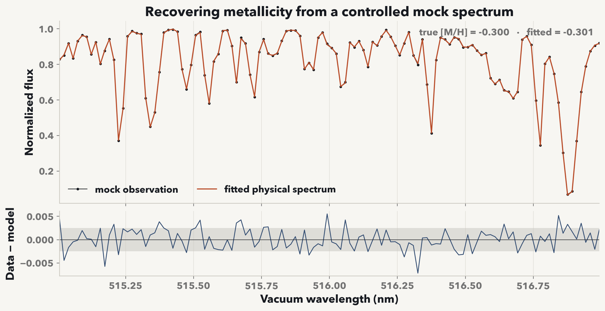
A controlled noisy mock spectrum and the fitted Payne Zero model, with the data-minus-model residual compared with the injected one-sigma noise — This controlled calculation uses the same one-label fitting interface demonstrated by the notebook. It synthesizes a spectrum at [M/H] = −0.300, adds Gaussian noise with 1σ = 0.0025, and starts at [M/H] = −0.050. Four bounded iterations recover [M/H] = −0.301. This is an internal-consistency example, not a measurement of accuracy on observed stars.

Fixed-atmosphere synthesis makes this repeated search practical. It identifies a candidate stellar state; it does not by itself establish that the candidate atmosphere satisfies the physical closure conditions.

Fit with a fixed atmosphere, then check the physical atmosphere

Converging a new atmosphere at every trial would spend most of the fit updating structures that will be discarded. The intended strategy separates exploration from acceptance. Repeated fixed-atmosphere synthesis evaluations first locate a candidate; the atmosphere solver is then called at that candidate, and the converged atmosphere is synthesized through the same instrument model and continuum treatment.

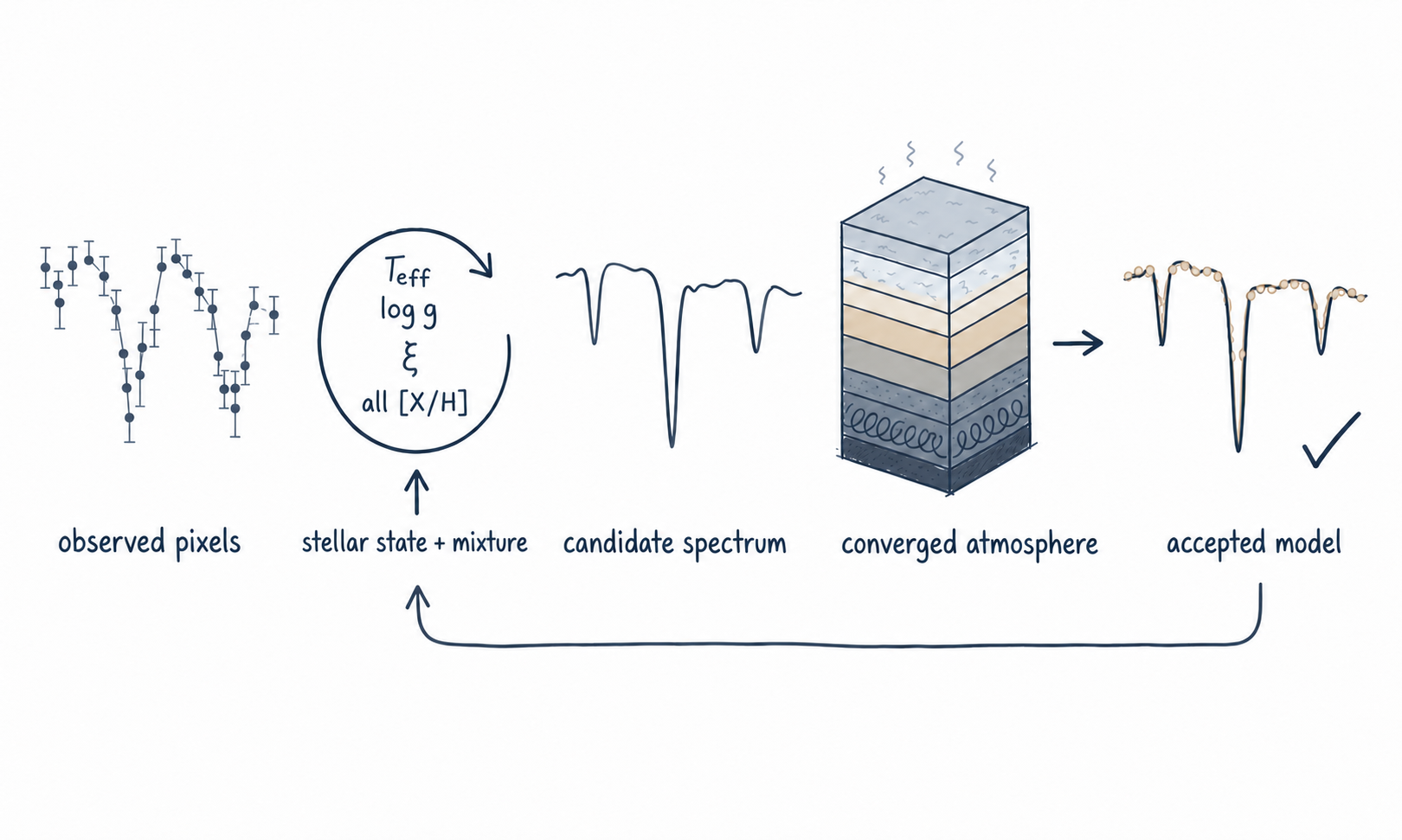
A fit of effective temperature, surface gravity, microturbulence, and element-by-element abundances followed by a converged-atmosphere evaluation and acceptance check — The search may use a grouped composition such as bulk metallicity and alpha enhancement, or independent element-to-hydrogen abundances [X/H]. Here ξ denotes microturbulent velocity. A separately converged atmosphere then tests whether convergence materially changes the flux or the fit before a result is retained.

refine_with_physical_atmosphere records two separate checks: whether the fixed-atmosphere and converged spectra agree within the configured tolerance after continuum profiling, and whether the converged model preserves the weighted fit statistic. If a material discrepancy remains, the fixed-atmosphere model proposes a small parameter correction within the allowed bounds. Another atmosphere is solved only when that correction is expected to improve the fit, and it is retained only if the converged model actually improves.

from tempfile import TemporaryDirectory

from fitter import (
    PhysicalAtmosphereConfiguration,
    refine_with_physical_atmosphere,
)
from payne_zero_atmosphere import solve_structured_atmosphere
from payne_zero_synthesis import synthesize

def converged_model(parameters):
    labels = {
        **solar_labels,
        "metallicity": float(parameters[0]),
    }
    with TemporaryDirectory() as directory:
        atmosphere_path = solve_structured_atmosphere(
            **labels,
            out_dir=directory,
        )
        return synthesize(
            atmosphere_path,
            wavelength_start_nm=500.0,
            wavelength_end_nm=502.0,
            resolution=300_000,
            spectral_operator=instrument,
            device=device,
            dtype=torch_dtype,
        ).normalized_flux

physical_result = refine_with_physical_atmosphere(
    observation,
    configuration,
    result,
    model,
    converged_model,
    PhysicalAtmosphereConfiguration(
        maximum_discrepancy_rms=2.0e-3,
        maximum_objective_degradation=0.1,
        minimum_predicted_objective_improvement=1.0e-3,
        maximum_physical_evaluations=4,
    ),
)
physical_result.save("runs/metallicity_fit_physical")

The final scientific product is therefore the model evaluated from a converged atmosphere. The earlier search result remains useful as a candidate and as a record of how the fitting routine reached that state, but it does not show that its atmosphere has converged.

APOGEE pixels require a wavelength-dependent instrument model

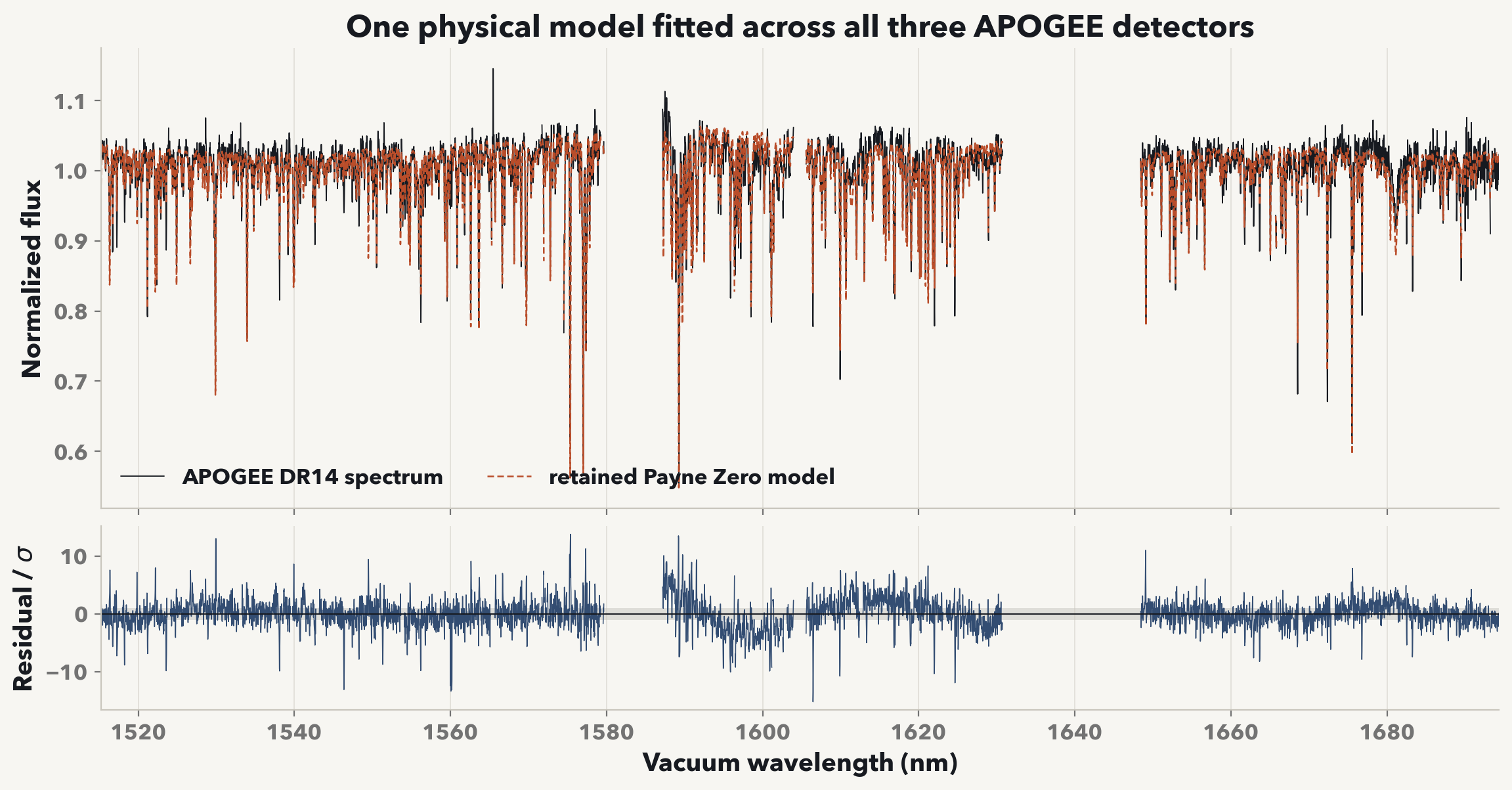
The packaged APOGEE DR14 example applies the same sequence to 7,514 retained pixels. In place of one constant resolving power, it uses a wavelength-dependent line-spread function, detector sampling, and the survey mask. It also fits a small residual velocity and an effective Gaussian broadening width, while solving a smooth multiplicative continuum independently on each detector.

The APOGEE helper fits effective temperature, surface gravity, bulk metallicity, alpha enhancement, and microturbulence; an option adds independent C, N, and O abundances. Use the generic fitter for a different element-by-element mixture. The packaged line-spread function is a representative DR14 all-slit mean, not an official visit-, fiber-, or star-specific ASPCAP kernel.

The notebook loads a packaged retained fit by default so the data preparation and model comparison can be inspected without rerunning the longer optimization. Setting PAYNE_ZERO_RUN_APOGEE=1 executes the fit on the packaged arrays. The displayed fit is a fresh execution with a fourth-order detector continuum. It uses the packaged H-band correction derived jointly from the solar and Arcturus atlases, so the stellar fit starts from line strengths already checked against two standard stars.

Profile the continuum during the stellar fit

The call below is already a joint stellar-parameter fit. The five values in reference_labels initialize effective temperature, surface gravity, bulk metallicity, alpha enhancement, and microturbulence; they are allowed to change during the fit. Residual velocity and Gaussian broadening are fitted as separate nuisance quantities.

The continuum coefficients are solved separately rather than treated as additional stellar parameters. At every trial spectrum, the fitter solves them by weighted linear least squares and then evaluates the residuals. The displayed example uses a fourth-order Legendre polynomial on each of the three detectors. Lower orders preserve more broad spectral shape; higher orders can absorb more normalization structure, so the order should be chosen before interpreting the stellar parameters.

import numpy as np
from fitter.apogee import fit_apogee_spectrum

with np.load("examples/data/apogee_dr14_example.npz") as spectrum:
    result = fit_apogee_spectrum(
        "runs/apogee_example",
        object_id="2M08002084+4044415",
        wavelength_nm=spectrum["wavelength_nm"],
        normalized_flux=spectrum["normalized_flux"],
        inverse_variance=spectrum["inverse_variance"],
        good_pixel_mask=spectrum["good_pixel_mask"],
        reference_labels=np.array(
            [4858.537, 2.426797, -0.3255714, 0.2527028, 1.278733]
        ),
        reference_vmacro_km_s=3.617606,
        synthesis_r_grid=300_000,
        continuum_order=4,
        fresh_jacobian_rounds=0,
        atomic_calibration_path=(
            "linelist_calibration/data/"
            "sun_arcturus_fts_hband_shared.npz"
        ),
        device="auto",
        dtype="auto",
        force=True,
    )

The executed Payne Zero model and an APOGEE DR14 giant spectrum across all three detector wavelength ranges, with residuals in units of the uncertainty used by the fit — An executed fit to APOGEE DR14 object 2M08002084+4044415 across all three detectors. Black is the observed spectrum and orange is the seven-parameter model: effective temperature, surface gravity, bulk composition, alpha enhancement, microturbulence, residual velocity, and Gaussian broadening. A fourth-order multiplicative continuum is solved separately on each detector at every stellar trial, and the shared solar–Arcturus H-band line correction is applied. The lower panel shows data minus model in units of each pixel's 1σ uncertainty as defined by the inverse variance used in the fit; the gray band marks ±1σ. The full wavelength range is shown rather than a selected line window.

The installed command accepts the same retained-pixel arrays:

payne-zero-fit-apogee \
  examples/data/apogee_dr14_example.npz \
  runs/apogee_example \
  --object-id 2M08002084+4044415 \
  --reference-labels 4858.537 2.426797 -0.3255714 0.2527028 1.278733 \
  --reference-vmacro 3.617606 \
  --synthesis-r-grid 300000 \
  --continuum-order 4 \
  --fresh-jacobian-rounds 0 \
  --atomic-calibration \
  linelist_calibration/data/sun_arcturus_fts_hband_shared.npz \
  --force

The command uses the default intrinsic grid density R = 300,000 before the APOGEE line-spread function and detector sampling. This R describes numerical wavelength sampling, not the delivered resolving power of the spectrograph.

Fit the stellar state and CNO abundances together

For a spectrum whose carbon, nitrogen, and oxygen pattern should not be tied to the bulk metal abundance, enable the extended fit. Payne Zero then varies the same five stellar quantities together with [C/M], [N/M], and [O/M]. These three logarithmic ratios measure carbon, nitrogen, and oxygen relative to the star's bulk metal abundance; the supplied values are starting points for the fit, not quantities held fixed. The instrument, continuum, and retained pixels are treated in the same way as in the preceding example.

import numpy as np
from fitter.apogee import fit_apogee_spectrum

with np.load("examples/data/apogee_dr14_example.npz") as spectrum:
    result = fit_apogee_spectrum(
        "runs/apogee_stellar_cno",
        object_id="2M08002084+4044415",
        wavelength_nm=spectrum["wavelength_nm"],
        normalized_flux=spectrum["normalized_flux"],
        inverse_variance=spectrum["inverse_variance"],
        good_pixel_mask=spectrum["good_pixel_mask"],
        # Starting values for Teff, log g, [M/H], [alpha/M], and vmicro.
        reference_labels=np.array(
            [4858.537, 2.426797, -0.3255714, 0.2527028, 1.278733]
        ),
        reference_vmacro_km_s=3.617606,
        fit_cno8=True,
        c_over_m=0.0,
        n_over_m=0.0,
        o_over_m=0.0,
        synthesis_r_grid=300_000,
        continuum_order=4,
        atomic_calibration_path=(
            "linelist_calibration/data/"
            "sun_arcturus_fts_hband_shared.npz"
        ),
        device="auto",
        dtype="auto",
        force=True,
    )

Fit individual abundances across an APOGEE sample

The full APOGEE application uses the same instrument and fitting machinery for 1,600 giants. [Fe/H] is the logarithmic iron-to-hydrogen ratio relative to the Sun. [X/Fe] states how one element X differs from the solar element-to-iron ratio. The calculation fits [Fe/H] and eleven independent [X/Fe] ratios—C, N, O, Mg, Al, Si, S, Ca, Ti, Mn, and Ni—while retaining the published DR14 effective temperature, surface gravity, and microturbulence in its main configuration. A sensitivity calculation also frees those three stellar quantities. Each accepted result is recalculated with a physically converged atmosphere.