Physics · Payne Zero

The two paths differ in the atmosphere supplied to synthesis

Spectrum synthesis requires a complete depth-dependent atmosphere. In every synthesis call, that atmospheric structure is held fixed while Payne Zero recomputes the chemical populations, continuous and line opacity, and radiative transfer for the requested composition and wavelength interval. The difference between the two model-generation paths is how the fixed structure was obtained.

For exploratory spectra and repeated parameter trials during a fit, Payne Zero predicts a starting atmospheric structure from the stellar parameters and abundances. The composition may be given as a bulk metallicity and alpha pattern, with carbon, nitrogen, and oxygen varied independently, or element by element. Synthesis can use that predicted structure immediately, but the product records that the atmosphere has not passed the convergence test. The speed comes from executing the physical synthesis efficiently; flux is not supplied by a label-to-flux emulator.

When the atmosphere is itself a result, or when a final spectrum must reflect a self-consistent response to the requested mixture, the atmosphere solver starts from the same prediction and iterates it first. Temperature, pressure, electron density, molecular balance, opacity, radiation, and convection are then allowed to respond to one another before the converged structure enters the same synthesis engine.

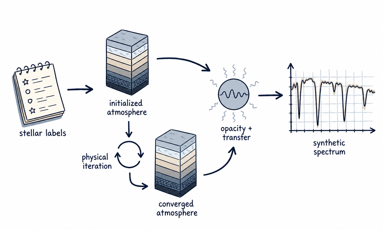
An initialized atmosphere entering synthesis either immediately while held fixed or after physical atmosphere convergence — Both paths calculate populations, opacity, and radiative transfer. Only the lower path corrects the atmospheric depth structure until its coupled physical state has converged.

The practical choice is therefore scientific rather than merely computational. Holding the initialized atmosphere fixed is useful for nearby trial spectra. Solving it is important when changes in composition or stellar parameters should also alter the temperature–pressure structure through line blanketing, molecular equilibrium, electron donation, or convection.

The calculation represents the atmosphere as a vertical column

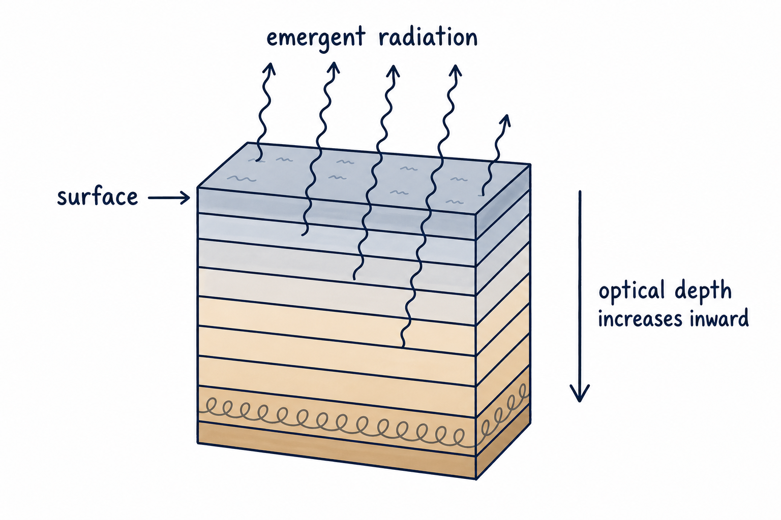
Payne Zero implements the one-dimensional, plane-parallel Kurucz atmosphere used in the paper under local thermodynamic equilibrium (LTE). The star is represented locally as horizontal layers: physical conditions change with depth, but not across the surface. The production grid contains 80 layers in Rosseland optical depth.

Six profiles summarize the structure that must be carried between iterations: column mass m, temperature T, gas pressure, electron density, Rosseland mean opacity, and radiative acceleration. The full solver state also carries the pressure, convection, population, and iteration quantities needed by the next physical pass. A converged product includes the populations and Doppler widths required by synthesis.

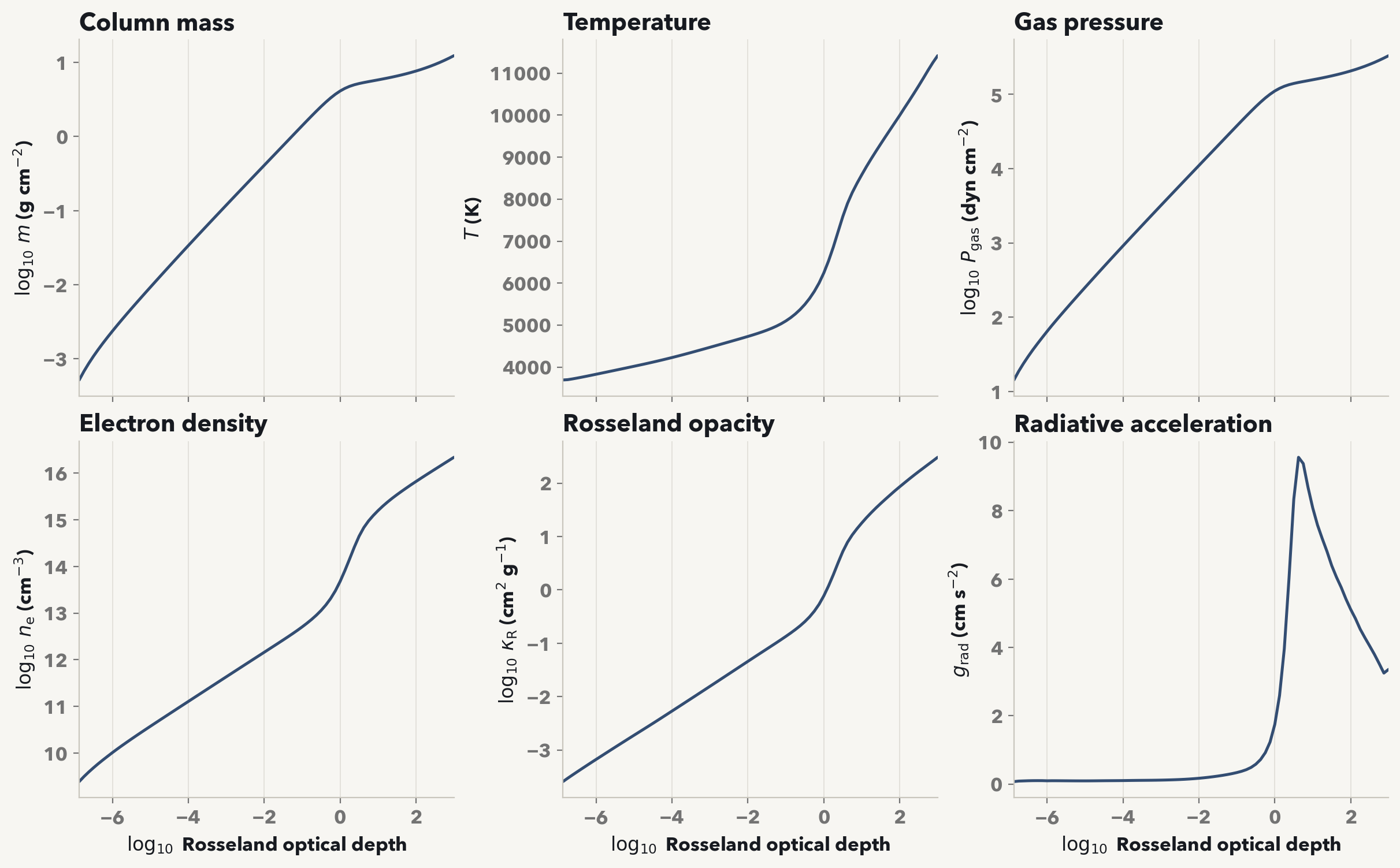
An actual solar starting atmosphere predicted by Payne Zero on its 80-layer Rosseland grid. These six coupled profiles are passed to the atmosphere solver; the solver then recomputes pressure, populations, opacity, radiation, convection, and the temperature correction until the convergence tests are met. The plotted state is an initialized atmosphere, not a flux prediction or a claim of convergence.

Column mass measures the material above a layer. Rosseland optical depth also accounts for how opaque that material is:

\mathrm{d}\tau_{\mathrm{R}} = \kappa_{\mathrm{R}}\,\mathrm{d}m

This mapping changes whenever temperature, pressure, or composition changes the mean opacity, so it is rebuilt as the atmosphere is corrected. Hydrostatic balance simultaneously relates gas and radiation pressure to the weight of the column.

A plane-parallel atmospheric column with optical depth increasing inward and radiation emerging from several layers — The atmosphere is one-dimensional but not uniform. The emergent radiation samples layers with different temperatures, populations, and opacities.

Stellar parameters provide the composition and a starting structure

Effective temperature sets the total energy flux the atmosphere must carry. Surface gravity enters hydrostatic balance. Microturbulence contributes to line widths and therefore affects both line blanketing and emergent profiles. The abundance inputs are expanded into a complete elemental mixture before the equation of state or opacity is evaluated.

Payne Zero accepts three abundance descriptions. A bulk [M/H] and [α/M] pattern is the ordinary choice. Carbon, nitrogen, and oxygen can instead vary independently for evolved or molecularly sensitive stars. An element-by-element interface accepts individual [X/H] values when a grouped pattern is not sufficient. These are different ways to describe the mixture used to construct the atmosphere; they do not select different population, opacity, or transfer physics.

Here the bracket notation is logarithmic relative to the Sun: [M/H] is the overall metal-to-hydrogen ratio, [X/H] is the ratio for one element X, and [α/M] is the shared alpha-element offset from the bulk metal pattern. One dex corresponds to a factor of ten.

The starting-atmosphere model predicts the six depth profiles together so their correlated changes are preserved. The bulk and independent-CNO inputs use a direct mapping from the requested stellar parameters. For an element-by-element mixture, each abundance is combined with its element identity before the depth structure is predicted. In every case the prediction contains atmospheric profiles, not a spectrum.

The prediction is useful because it usually begins closer to the physical solution than a generic grey atmosphere. It is still only a start. The code reconstructs the remaining state around those profiles, and only the repeated physical atmosphere cycle can show that the structure has converged. In particular, the element-by-element starting structure is treated as provisional for rapid spectrum trials; a retained atmosphere for that mixture must pass the exact convergence cycle.

Local conditions determine which absorbers are present

LTE assumes that the local temperature and pressure determine the excitation and ionization populations even though radiation still travels between layers. At each layer, the equation of state solves charge conservation, Saha ionization, Boltzmann excitation, and molecular equilibrium. The result is the density of each ionization stage, excitation level, and molecule. A transition can be present in the catalog yet contribute almost no opacity when its lower level has negligible population in that layer.

Molecules make abundance responses coupled rather than element-by-element. In a cool atmosphere, CO can bind much of the available carbon or oxygen; CN and OH then respond to what remains. Changing one abundance can therefore alter several molecular systems at once.

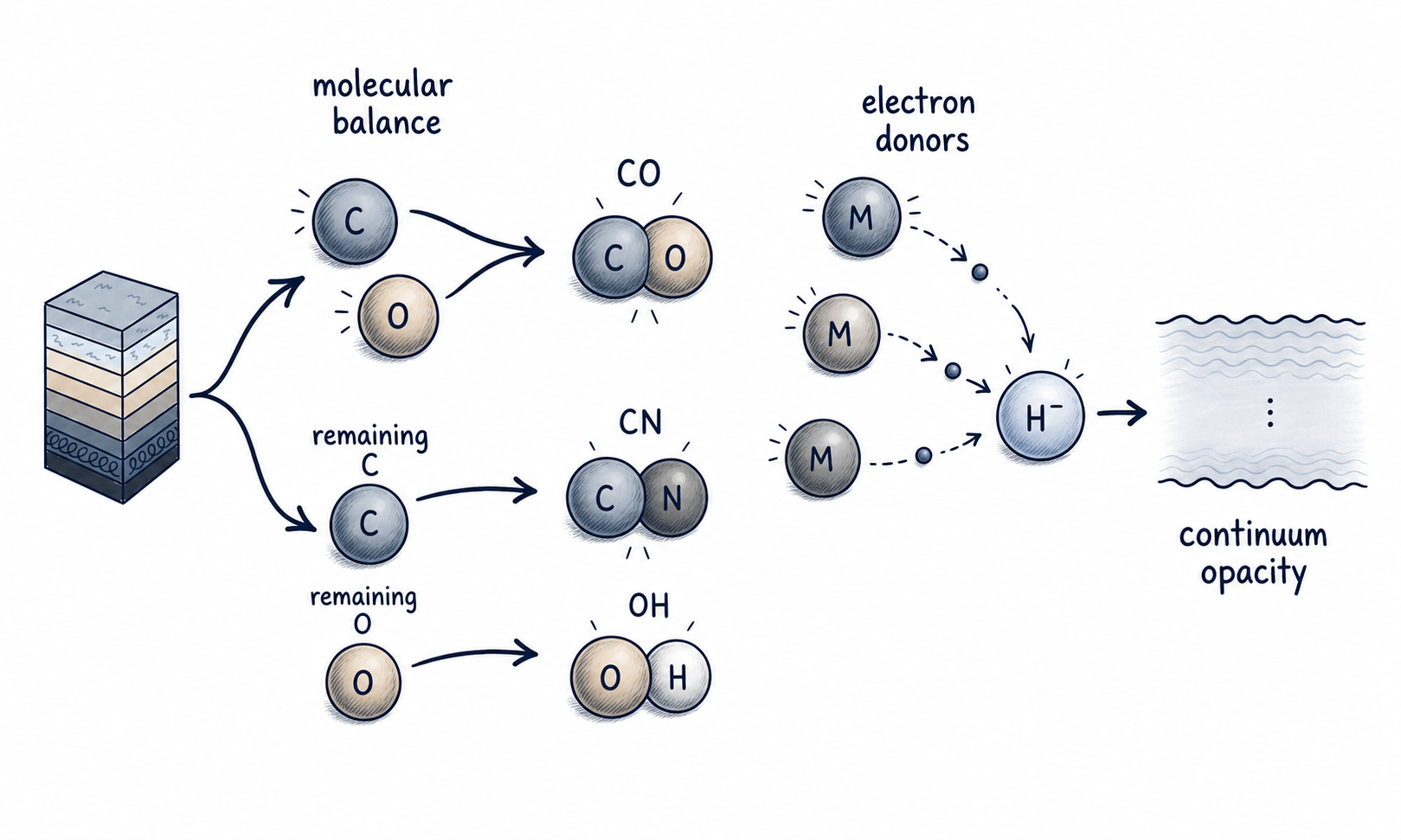
Carbon and oxygen forming CO before the remaining carbon and oxygen enter CN and OH, alongside electron donors feeding H-minus opacity — CO couples the carbon and oxygen inventories, while CN and OH respond to the atoms left after that balance. Electron donors provide another indirect path by changing the H⁻ continuum.

Electron donors provide a second connection. Their abundances change electron density and can therefore change H⁻ continuous opacity. Lines from unrelated species can appear stronger or weaker because the reference continuum moved. Populations and continuous opacity must consequently be rebuilt together for every requested mixture.

Those populations become continuous and line extinction

At each wavelength and depth, total extinction combines continuous absorption, continuous scattering, and all active lines:

\chi_\nu = \kappa_{\nu,\mathrm{c}} + \sigma_{\nu,\mathrm{c}} + \sum_l \kappa_{\nu,l}

The continuous calculation includes the principal bound-free and free-free processes from hydrogen, helium, and metals. H⁻ supplies much of the optical and near-infrared continuum in cool stars. Rayleigh and electron scattering remain separate from thermal absorption because they enter the source function differently.

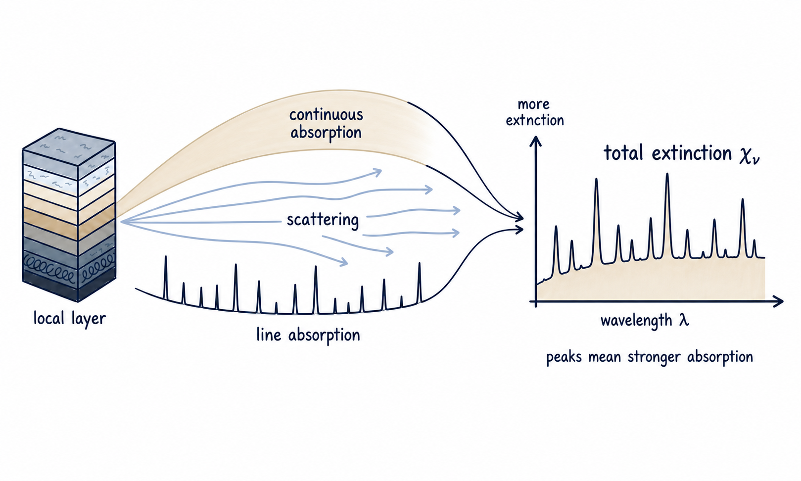
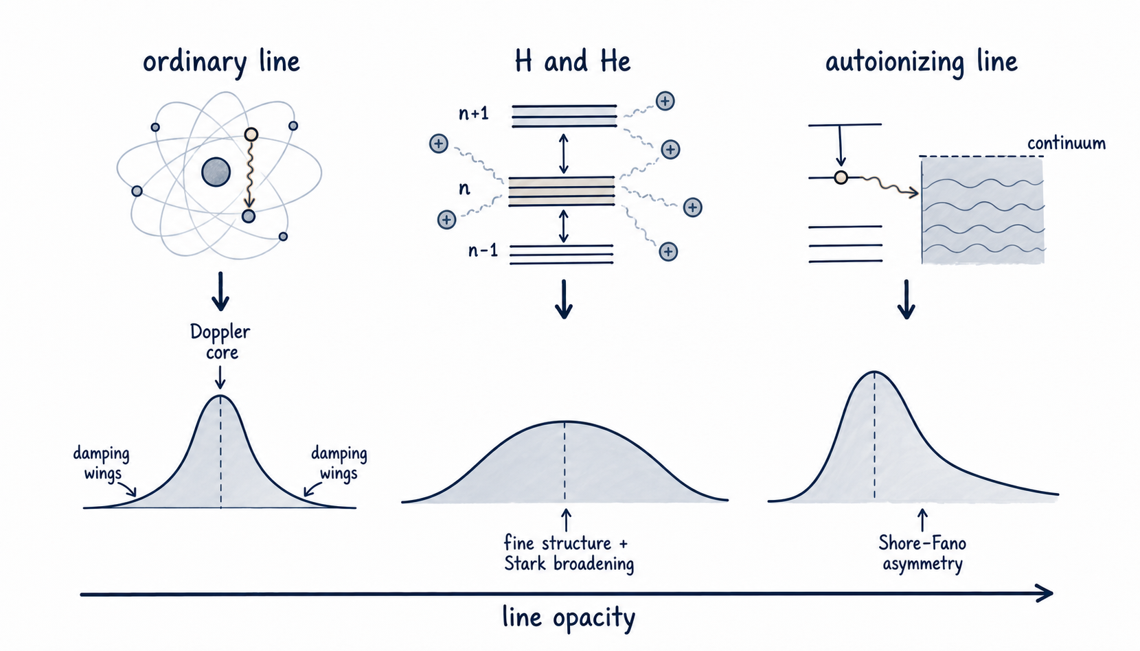
Continuous absorption, scattering, and line absorption combining into total extinction, with an axis showing that upward peaks mean stronger absorption — Continuous absorption, scattering, and active lines are evaluated at the same local depth state and added before radiative transfer. The peaks point upward because this panel shows extinction; they indicate stronger absorption, not emergent emission.

For an ordinary LTE transition, the lower-level population and oscillator strength set the integrated line opacity. Its normalized profile distributes that opacity in frequency. Thermal motion and microturbulence set the Doppler width,

\Delta v_{\mathrm{D}}^2 = \frac{2k_{\mathrm{B}}T}{m_l} + \xi^2

while radiative, Stark, and van der Waals damping determine the wings. Ordinary lines use a Voigt profile. Payne Zero also retains the required specialized Kurucz branches for hydrogen fine structure and Stark profiles, high-series dissolution through occupation probabilities, He I, ³He, He II, and asymmetric Shore–Fano autoionizing profiles. Molecular masses set the thermal widths of molecular transitions.

Most transitions use a Voigt profile. Hydrogen and helium use specialized broadening where required, and autoionizing transitions use an asymmetric Shore–Fano profile.

Radiative transfer converts extinction into emergent flux

Extinction defines monochromatic optical depth through the column. In LTE, line and continuous absorption contribute thermal emission through the Planck function. Continuum scattering depends on the mean radiation field, so it is iterated rather than treated as purely local emission:

S_\nu = \epsilon_\nu B_\nu(T) + \left(1-\epsilon_\nu\right)J_\nu

The transfer equation then follows the specific intensity along each ray through all layers, where μ is the direction cosine:

\mu\,\frac{\mathrm{d}I_\nu}{\mathrm{d}\tau_\nu} = I_\nu - S_\nu

Depths remain coupled at one wavelength because a ray traverses the complete column. One wavelength does not directly depend on the next, which later provides the large parallel dimension in synthesis.

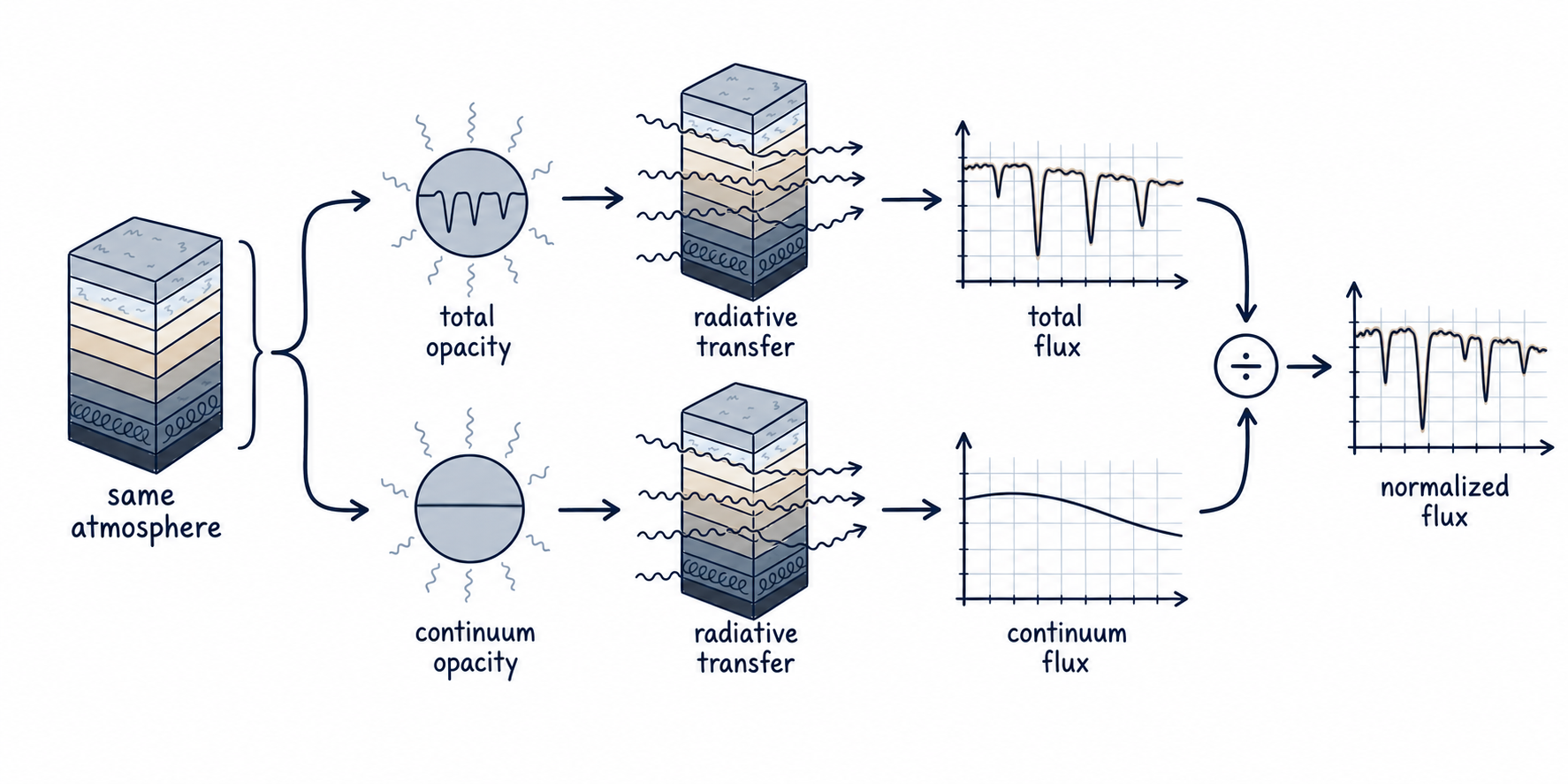
Payne Zero solves total and physical-continuum transfer together. The returned arrays contain total surface flux density per nanometer, continuum surface flux density, and their normalized ratio. When an instrument model is supplied, total and continuum flux receive the same velocity shift, broadening, line-spread function, and sampling before their ratio is formed on observed pixels.

The same atmosphere passing through total-opacity and continuum-opacity transfer branches to produce total, continuum, and normalized flux — Total and continuum branches share the same atmospheric structure and geometry. Keeping both physical fluxes makes normalization and instrument projection consistent.

The atmosphere solver feeds radiation back into the structure

Fixed-atmosphere synthesis stops after the transfer calculation. Atmosphere convergence cannot, because the radiation field determines radiative acceleration and the radiative share of the energy flux. Those quantities must update pressure, temperature, and column mass before populations and opacity are rebuilt.

One outer pass evaluates hydrostatic balance and the equation of state, rebuilds opacity, solves transfer over the atmosphere's opacity-sampling frequencies, evaluates radiative pressure and convection, applies a temperature correction, and remaps the corrected profiles to the standard Rosseland grid. The next pass begins from that remapped state. Later stages consume quantities calculated earlier in the same pass, so this order cannot be rearranged into independent atmosphere iterations.

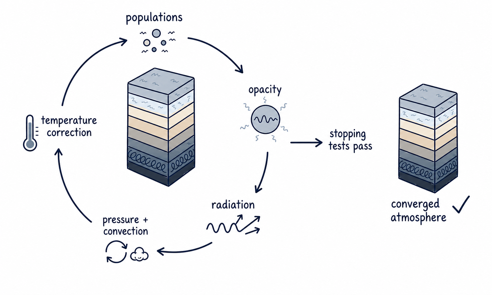
The ordered Payne Zero atmosphere cycle from populations through opacity, radiation, pressure and convection, temperature correction, and closure tests — One physical pass follows this order. Its corrected structure becomes the input to the next pass until the stopping criteria are met.

The temperature correction seeks the flux implied by the requested effective temperature. Radiation and convection together must carry that energy through the atmosphere:

F_{\mathrm{rad}} + F_{\mathrm{conv}} = \sigma_{\mathrm{SB}}\,T_{\mathrm{eff}}^4

The production stopping test monitors whether the deep temperature structure has ceased changing after the required minimum passes; the recorded flux diagnostics provide a separate check on the resulting energy balance. A learned starting structure can reduce the number of passes, but it does not replace any physical stage or satisfy the stopping test by itself.

Atmosphere passes are ordered; wavelengths are synthesized in parallel

Atmosphere passes are sequential, but expensive work inside one pass can be divided over depth, transitions, and opacity-sampling frequencies. Payne Zero uses Numba-compiled multicore CPU kernels for those blocks while preserving the ordered outer correction cycle. Fixed tables and catalogs remain in typed in-process arrays rather than being repeatedly staged through intermediate files.

Synthesis exposes much broader parallelism once the atmosphere is fixed. PyTorch evaluates batches of independent wavelength columns and active line profiles on CUDA, Apple Metal, or CPU, keeping depth–wavelength arrays and fixed transfer geometry resident until the final flux is returned. Atmosphere-dependent populations, opacity, and flux are still recomputed for every stellar state; no synthetic flux is cached or emulated.

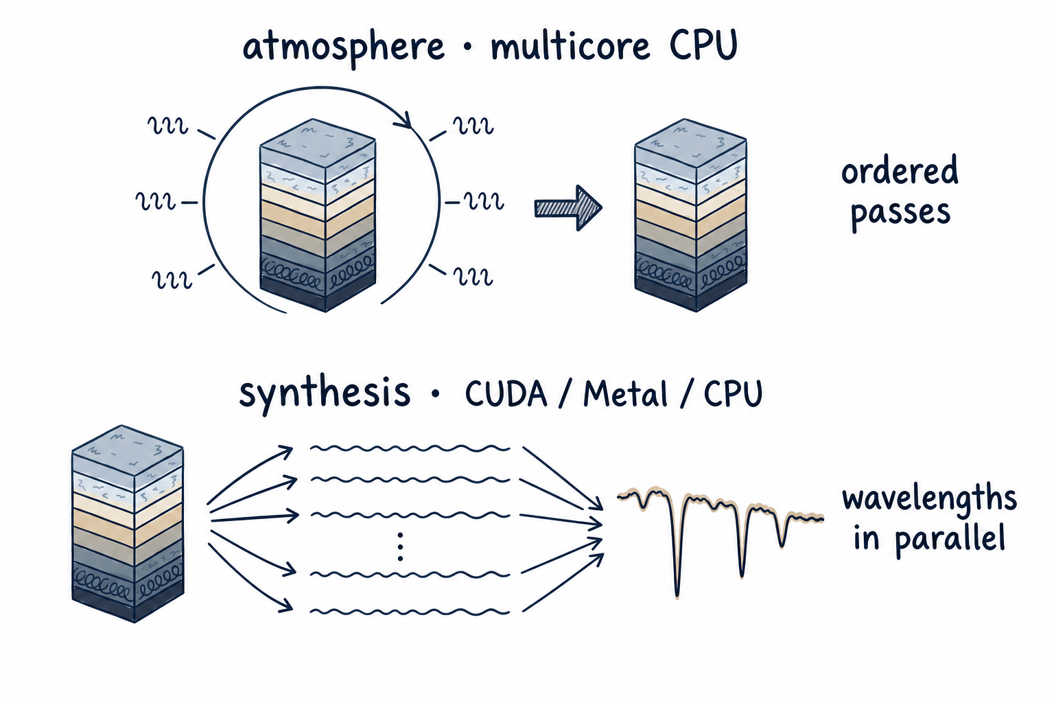
Ordered atmosphere passes using multicore CPU work alongside wavelength-parallel spectrum synthesis on CUDA, Apple Metal, or CPU — The atmosphere and synthesis engines use different hardware layouts because their physical dependencies are different: ordered correction passes for structure, and many independent wavelength columns for a fixed atmosphere.

A structured atmosphere archive is the handoff between these two packages. It carries the complete abundance mixture, depth arrays, units, convergence state, and source information. The synthesis package checks that structure before using the atmosphere, so a saved model and an in-memory one contain the same required fields.

Know the physical assumptions and their limits

The model is one-dimensional, plane-parallel, and LTE. The atmosphere path does not include optional non-LTE or turbulent-pressure branches from the broader historical code family. It also does not remove departures caused by three-dimensional convection, chromospheres, non-LTE line formation, incomplete or inaccurate line data, or an incorrect instrument model.

Some cool, high-gravity molecular atmospheres enter an unstable fixed-point regime in both the original Kurucz calculation and Payne Zero. Small temperature changes can reorganize molecules, opacity, the equation of state, and convection together. A failure to converge in that regime should be diagnosed rather than relabeled as a converged atmosphere.

These boundaries are why products retain convergence and source metadata, and why a new stellar or instrumental regime should be checked against appropriate reference calculations. A standard-star line correction remains conditional on the adopted atmosphere, abundances, masks, and instrument model; it is not a laboratory measurement.

Fit an observed spectrumContinue from a generated spectrum to instrument matching, weighted fitting, and the converged-atmosphere check.